arviz_plots.plot_psense_quantities

arviz_plots.plot_psense_quantities(dt, alphas=None, quantities=None, mcse=True, var_names=None, filter_vars=None, prior_var_names=None, likelihood_var_names=None, prior_coords=None, likelihood_coords=None, coords=None, sample_dims=None, plot_collection=None, backend=None, labeller=None, aes_by_visuals=None, visuals=None, **pc_kwargs)

Plot power scaled posterior quantities.

The posterior quantities are computed by power-scaling the prior or likelihood and visualizing the resulting changes, using Pareto-smoothed importance sampling to avoid refitting as explained in [1].

Parameters:

dtxarray.DataTree

Input data

alphastuple of float

Lower and upper alpha values for power scaling. Defaults to (0.8, 1.25).

quantitieslist of str

Quantities to plot. Options are ‘mean’, ‘sd’, ‘median’. For quantiles, use ‘0.25’, ‘0.5’, etc. Defaults to [‘mean’, ‘sd’].

mcsebool

Whether to plot the Monte Carlo standard error for each quantity. Defaults to True.

var_namesstr or list of str, optional

One or more variables to be plotted. Prefix the variables by ~ when you want to exclude them from the plot.

filter_vars{None, “like”, “regex”}, optional, default=None

If None (default), interpret var_names as the real variables names. If “like”, interpret var_names as substrings of the real variables names. If “regex”, interpret var_names as regular expressions on the real variables names.

prior_var_namesstr, optional.

Name of the log-prior variables to include in the power scaling sensitivity diagnostic

likelihood_var_namesstr, optional.

Name of the log-likelihood variables to include in the power scaling sensitivity diagnostic

prior_coordsdict, optional.

Coordinates defining a subset over the group element for which to compute the log-prior sensitivity diagnostic

likelihood_coordsdict, optional

Coordinates defining a subset over the group element for which to compute the log-likelihood sensitivity diagnostic

coordsdict, optional

sample_dimsstr or sequence of hashable, optional

Dimensions to reduce unless mapped to an aesthetic. Defaults to rcParams["data.sample_dims"]

plot_collectionPlotCollection, optional

backend{“matplotlib”, “bokeh”, “plotly”}, optional

labellerlabeller, optional

aes_by_visualsmapping of {strsequence of str}, optional

Mapping of visuals to aesthetics that should use their mapping in plot_collection when plotted. Valid keys are the same as for visuals.

visualsmapping of {strmapping or bool}, optional

Valid keys are:

• prior_markers -> passed to scatter_xy

• prior_lines -> passed to line_xy

• likelihood_markers -> passed to scatter_xy

• likelihood_lines -> passed to line_xy

• mcse -> passed to hline

• ticks -> passed to set_xticks

• title -> passed to labelled_title

• legend -> passed to arviz_plots.PlotCollection.add_legend

**pc_kwargs

Passed to arviz_plots.PlotCollection.grid

Returns:

PlotCollection

References

[1]

Kallioinen et al, Detecting and diagnosing prior and likelihood sensitivity with power-scaling, Stat Comput 34, 57 (2024), https://doi.org/10.1007/s11222-023-10366-5

Examples

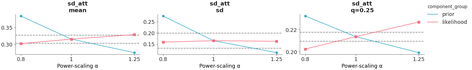
Select a single parameter, one of the two likelihoods, and plot the mean, standard deviation, and 25th percentile.

>>> from arviz_plots import plot_psense_quantities, style
>>> style.use("arviz-variat")
>>> from arviz_base import load_arviz_data
>>> rugby = load_arviz_data('rugby')
>>> plot_psense_quantities(rugby,
>>>                        var_names=["sd_att"],
>>>                        likelihood_var_names=["home_points"],
>>>                        quantities=["mean", "sd", "0.25"])

The posterior quantities are computed by power-scaling the prior or likelihood and visualizing the resulting changes. Sensitivity can then be quantified by considering how much the perturbed quantities differ from the base quantities.

Sensitivity posterior quantities

Sensitivity posterior quantities